Post-processing

MapReader post-processing’s sub-package currently contains two post-processing methods:

Context based post-processing - for improving predictions of continuous features such as railways, roads, coastlines, etc.
Occlusion analysis - for better understanding the model’s predictions.

For both of these methods, you will need to have saved the predictions following the instructions in /using-mapreader/step-by-step-guide/4-classify.

Context Post-processing

MapReader’s context based post-processing is based on the idea that features such as railways, roads, coastlines, etc. are continuous and so patches with these labels should be found near to other patches also with these labels. For example, if a patch is predicted to be a railspace, but is surrounded by patches predicted to be non-railspace, then it is likely that the railspace patch is a false positive.

To implement this, for a given patch, the code checks whether any of the 8 surrounding patches have the same label (e.g. ‘railspace’) and, if not, assumes the current patch’s predicted label to be a false positive. The user can then choose how to relabel the patch (e.g. ‘railspace’ -> ‘no’).

If you have your predictions saved in a csv file, you will first need to load them into a pandas DataFrame:

import pandas as pd

preds = pd.read_csv("path/to/predictions.csv", index_col=0)

You can then run the context post-processing code as follows:

from mapreader.process.context_post_process import ContextPostProcessor

labels_map = {
    0: "no",
    1: "railspace",
    2: "building",
    3: "railspace&building"
}

patches = ContextPostProcessor(preds, labels_map=labels_map)

This context based post-processing will only work for features that are expected be continuous (e.g. railway, road, coastline, etc.) or clustered (e.g. a large body of water). You will need to tell MapReader which labels to select and then get the context for each of the relevant patches in order to work out if it is isolated or part of a line/cluster.

For example, if you want to post-process patches which are predicted to be ‘railspace’ or ‘railspace&building’, you would do the following:

labels=["railspace", "railspace&building"]
patches.get_context(labels=labels)

Note

In the above example, we needed to use both ‘railspace’ and ‘railspace&building’ as our labels, since the continuous feature we are trying to post-process is railway lines (included in both these labels).

You will also need to tell MapReader how to update the label of each patch that is isolated and therefore likely to be a false positive. This is done using the remap argument, which takes a dictionary of the form {old_label: new_label}.

For example, if you want to remap all isolated ‘railspace’ patches to be labelled as ‘no’, and all isolated ‘railspace&building’ patches to be labelled as ‘building’, you would do the following:

remap={"railspace": "no", "railspace&building": "building"}
patches.update_preds(remap=remap)

By default, only patches with model confidence of below 0.7 will be relabelled. You can adjust this by passing the conf argument.

e.g. to relabel all isolated patches with confidence below 0.9, you would do the following:

remap={"railspace": "no", "railspace&building": "building"}
patches.update_preds(remap=remap, conf=0.9)

Instead of relabelling your chosen patches to an existing label, you can also choose to relabel them to a new label. For example, to mark them as ‘false_positive’, you would do the following:

remap={"railspace": "false_positive", "railspace&building": "false_positive"}
patches.update_preds(remap=remap)

By default, after running update_preds, a new column will be added to your patches DataFrame called “new_predicted_label”. This will contain the updated predictions (or NaN if the patch was not relabelled).

Alternatively, to save the updated predictions inplace you can pass the inplace argument:

remap={"railspace": "no", "railspace&building": "building"}
patches.update_preds(remap=remap, inplace=True)

Finally, to save your outputs to a csv file, you can do the following:

patches.to_csv("path/to/save/updated_predictions.csv")

Occlusion Analysis

Occlusion analysis is a method for understanding the model’s predictions by occluding parts of the input image and observing the effect on the model’s output. This can help to identify which parts of the image are most important for the model’s predictions.

First, to set up your analyzer, you will need to load your predictions and your model. You can do this by passing the path to your predictions csv file and the path to your model.pth file as follows:

from mapreader.process.occlusion_analysis import OcclusionAnalyzer

analyzer = OcclusionAnalyzer(
    patch_df="path/to/predictions.csv",
    model="path/to/model.pth",
)

Or, if you have already loaded your predictions into a pandas DataFrame, you can pass this directly:

analyzer = OcclusionAnalyzer(
    patch_df=preds,
    model="path/to/model.pth",
)

If you have uploaded your model to an online repository (e.g. HuggingFace) and do not have the model.pth file, you can load the model and it in as a torch.nn.Module object. e.g. for our `railspace model<https://huggingface.co/Livingwithmachines/mr_resnest101e_finetuned_OS_6inch_2nd_ed>`__:

import timm
from mapreader.process.occlusion_analysis import OcclusionAnalyzer

model = timm.create_model("hf_hub:Livingwithmachines/mr_resnest101e_finetuned_OS_6inch_2nd_ed", pretrained=True)
analyzer = OcclusionAnalyzer(
    patch_df=preds,
    model=model,
)

You can set the model device using the device argument. By default, the device will be set to “cuda” if available, otherwise “cpu”.

e.g. to set the device to “cpu”, you would do the following:

analyzer = OcclusionAnalyzer(
    patch_df="path/to/predictions.csv",
    model="path/to/model.pth",
    device="cpu",
)

Once you have set up your analyzer, you should set a loss function to use for the occlusion analysis. e.g. to use PyTorch’s cross-entropy loss function as your loss function, you can pass the string “cross-entropy” as the loss_fn argument:

#EXAMPLE
analyzer.add_loss_fn("cross-entropy")

Note

Implemented options for the loss function are “cross-entropy” (default), “bce” (binary cross-entropy) and “mse” (mean squared error).

Alternatively, if you would like to use a loss function other than those implemented, you can pass any torch.nn loss function as the loss_fn argument.

e.g. to use the mean absolute error as your loss function:

#EXAMPLE
from torch import nn
loss_fn = nn.L1Loss()

analyzer.add_loss_fn(loss_fn)

Once this is set up, you can run the occlusion analysis as follows:

#EXAMPLE
results = analyzer.run_occlusion(
    label="railspace"
    sample_size=10
    )

The above example shows how to run the occlusion analysis on a random sample of 10 patches predicted as “railspace”. The results will be a list of images showing the occlusion effect on the model’s predictions. e.g.:

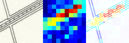
By default, the occlusion block will be 14 pixels by 14 pixels. You may want to adjust this based on the size of your patches or the desired “resolution” of your results. You can adjust this by passing the block_size argument:

e.g. to set the occlusion block to be 20 pixels by 20 pixels:

#EXAMPLE
results = analyzer.run_occlusion(
    label="railspace"
    sample_size=10,
    block_size=20
    )

Note

If you use smaller block size, the occlusion analysis will be more granular but will take longer to run.

If you’d like to save the results to a folder, you can pass the save and path_save arguments when running the occlusion analysis:

#EXAMPLE
analyzer.run_occlusion(
    label="railspace"
    sample_size=10,
    save=True,
    path_save="path/to/save/results"
    )

This will no longer return a list of images but instead will save the images to the specified folder.