Load

Note

Run these commands in a Jupyter notebook (or other IDE), ensuring you are in your mr_py38 python environment.

Note

You will need to update file paths to reflect your own machines directory structure.

MapReader’s Load subpackage is used to load, visualize and patchify images (e.g. maps) saved locally.

Load images (and metadata)

First, images (e.g. png, jpeg, tiff or geotiff files) can be loaded in using MapReader’s loader() function.

This can be done using:

from mapreader import loader

my_files = loader("./path/to/files/*.png")

or

from mapreader import loader

my_files = loader("./path/to/files/", file_ext="png")

For example, if you have downloaded your maps using the default settings of our Download subpackage or have set up your directory as recommended in our Input Guidance:

#EXAMPLE
my_files = loader("./maps/*.png")

or

#EXAMPLE
my_files = loader("./maps", file_ext="png")

The loader function creates a MapImages object (my_files) which contains information about your map images. To see the contents of this object, use:

print(my_files)

You will see that your MapImages object contains the files you have loaded and that these are labelled as ‘parents’.

If your image files are georeferenced and already contain metadata (e.g. geoTIFFs), you can add this metadata into your MapImages object using:

my_files.add_geo_info()

Note

This function will reproject your coordinates into “EPSG:4326”. To change this specify target_crs.

Or, if you have separate metadata (e.g. a csv, xls or xlsx file or, a pandas dataframe), use:

my_files.add_metadata(metadata="./path/to/metadata.csv")

Note

Specific guidance on preparing your metadata file/dataframe can be found on our Input Guidance page.

For example, if you have downloaded your maps using the default settings of our Download subpackage or have set up your directory as recommended in our Input Guidance </Input-guidance>:

#EXAMPLE
my_files.add_metadata(metadata="./maps/metadata.csv")

Advanced usage

Other arguments you may want to specify when adding metadata to your images include:

index_col - By default, this is set to 0 so the first column of your csv/excel spreadsheet will be used as the index column when creating a pandas dataframe. If you would like to use a different column you can specify index_col.
columns - By default, the add_metadata() method will add all the columns in your metadata to your MapImages object. If you would like to add only specific columns, you can pass a list of these as the columnss argument (e.g. columns=[`name`, `coordinates`, `region`]) to add only these columns to your MapImages object.
ignore_mismatch- By default, this is set to False so that an error is given if the images in your MapImages object are mismatched to your metadata. Setting ignore_mismatch to True (by specifying ignore_mismatch=True) will allow you to bypass this error and add mismatched metadata. Only metadata corresponding to images in your MapImages object will be added.
delimiter - By default, this is set to |. If your csv file is delimited using a different delimiter you should specify the delimiter argument.

Note

In MapReader versions < 1.0.7, coordinates were miscalculated. To correct this, use the add_coords_from_grid_bb() method to calculate new, correct coordinates.

Patchify

Once you’ve loaded in all your data, you’ll then need to ‘patchify’ your images.

Creating patches from your parent images is a core intellectual and technical task within MapReader. Choosing the size of your patches (and whether you want to measure them in pixels or in meters) is an important decision and will depend upon the research question you are trying to answer:

Smaller patches (e.g. 50m x 50m) tend to work well on very large-scale maps (like the 25- or 6-inch Ordnance Survey maps of Britain).
Larger patches (500m x 500m) will be better suited to slightly smaller-scale maps (for example, 1-inch Ordnance Survey maps).

In any case, the patch size you choose should roughly match the size of the visual feature(s) you want to label. Ideally your features should be smaller (in any dimension) than your patch size and therefore fully contained within a patch.

To patchify your maps, use:

my_files.patchify_all()

By default, this slices images into 100 x 100 pixel patches which are saved as .png files in a newly created directory called ./patches_100_pixel (here, 100 represents the patch_size and pixel represents the method used to slice your parent images).

If you are following our recommended directory structure, after patchifying, your directory should look like this:

project
├──your_notebook.ipynb
└──maps
│   ├── map1.png
│   ├── map2.png
│   ├── map3.png
│   ├── ...
│   └── metadata.csv
└──patches_100_pixel
    ├── patch-0-100-#map1.png#.png
    ├── patch-100-200-#map1.png#.png
    ├── patch-200-300-#map1.png#.png
    └── ...

If you would like to change where your patches are saved, you can change this by specifying path_save.

e.g:

#EXAMPLE
my_files.patchify_all(path_save="./maps/my_patches_dir")

This will create the following directory structure:

project
├──your_notebook.ipynb
└──maps
    ├── map1.png
    ├── map2.png
    ├── map3.png
    ├── ...
    ├── metadata.csv
    └── my_patches_dir
         ├── patch-0-100-#map1.png#.png
         ├── patch-100-200-#map1.png#.png
         ├── patch-200-300-#map1.png#.png
         └── ...

If you would like to change the size of your patches, you can specify patch_size.

e.g. to slice your maps into 500 x 500 pixel patches:

#EXAMPLE
my_files.patchify_all(patch_size=500)

This will save your patches as .png files in a directory called patches_500_pixel.

Note

You can combine the above options to change both the directory name in which patches are saved and patch size.

Providing you have loaded geographic coordinates into your MapImages object, you can also specify method = "meters" to slice your images by meters instead of pixels.

e.g. to slice your maps into 50 x 50 meter patches:

#EXAMPLE
my_files.patchify_all(method="meters", patch_size=50)

This will save your patches as .png files in a directory called patches_50_meters. As above, you can use the path_save argument to change where these patches are saved.

Advanced usage

Other arguments you may want to specify when patchifying your images include:

square_cuts - By default, this is set to False. Thus, if your patch_size is not a factor of your image size (e.g. if you are trying to slice a 100x100 pixel image into 8x8 pixel patches), you will end up with some rectangular patches at the edges of your image. If you set square_cuts=True, then all your patches will be square, however there will be some overlap between edge patches. Using square_cuts=True is useful if you need square images for model training, and don’t want to warp your rectangular images by resizing them at a later stage.
add_to_parent - By default, this is set to True so that each time you run patchify_all() your patches are added to your MapImages object. Setting it to False (by specifying add_to_parent=False) will mean your patches are created, but not added to your MapImages object. This can be useful for testing out different patch sizes.
rewrite - By default, this is set to False so that if your patches already exist they are not overwritten. Setting it to True (by specifying rewrite=True) will mean already existing patches are recreated and overwritten.

If you would like to save your patches as geo-referenced tiffs (i.e. geotiffs), use:

my_files.save_patches_as_geotiffs()

This will save each patch in your MapImages object as a georeferenced .tif file in your patches directory.

Note

MapReader also has a save_parents_as_geotiff() method for saving parent images as geotiffs.

After running the patchify_all() method, you’ll see that print(my_files) shows you have both ‘parents’ and ‘patches’. To view an iterable list of these, you can use the list_parents() and list_patches() methods:

parent_list = my_files.list_parents()
patch_list = my_files.list_patches()

print(parent_list)
print(patch_list[0:5])  # too many to print them all!

Having these list saved as variables can be useful later on in the pipeline.

It can also be useful to create dataframes from your MapImages objects. To do this, use:

parent_df, patch_df = my_files.convert_images()

Then, to view these, use:

parent_df

or

patch_df

Note

These parent and patch dataframes will not automatically update so you will want to run this command again if you add new information into your MapImages object.

At any point, you can also save these dataframes by passing the save argument to the convert_images() method:

parent_df, patch_df = my_files.convert_images(save=True)

By default, this will save your parent and patch dataframes as parent_df.csv and patch_df.csv respectively.

If instead, you’d like to save them as excel files, add save_format="excel" to your command:

parent_df, patch_df = my_files.convert_images(save=True, save_format="excel")

Alternatively, you can save your patch metadata in a georeferenced json (i.e. geojson) file. To do this, use:

my_files.save_patches_to_geojson()

By default, this will save all the metadata for your patches in a newly created patches.geojson file.

Note

The patch images are not saved within this file, only the metadata and patch coordinates.

Visualize (optional)

To view a random sample of your images, use:

my_files.show_sample(num_samples=3)

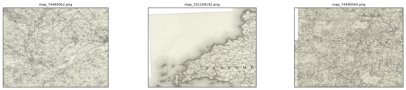
By default, this will show you a random sample of your parent images.

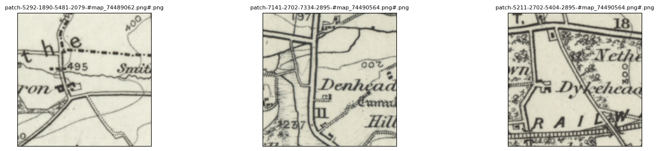
If, however, you want to see a random sample of your patches use the tree_level="patch" argument:

my_files.show_sample(num_samples=3, tree_level="patch")

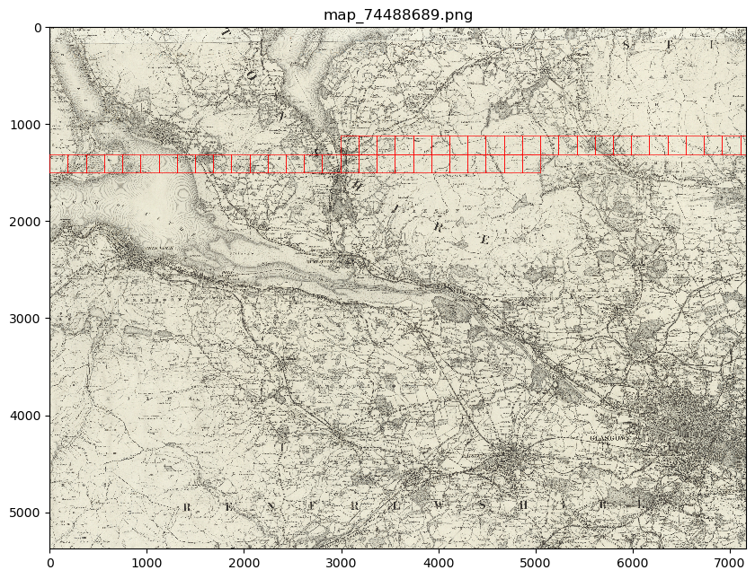
It can also be helpful to see your patches in the context of their parent image. To do this use the show() method.

e.g. :

#EXAMPLE
patch_list = my_files.list_patches()
my_files.show(patch_list[250:300])

or

#EXAMPLE
patch_list = my_files.list_patches()
files_to_show = [patch_list[0], patch_list[350], patch_list[400]]
my_files.show(files_to_show)

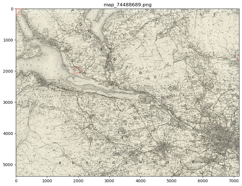
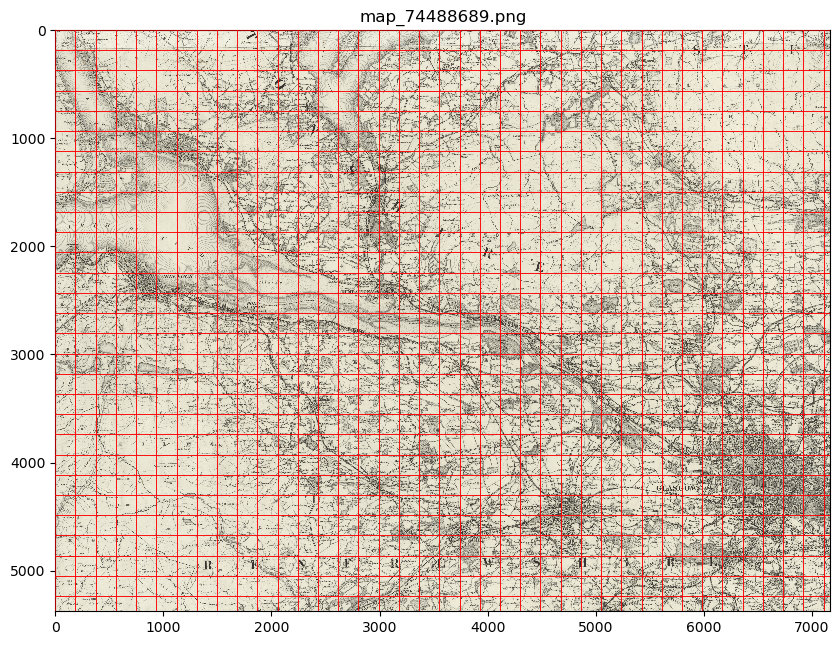
This will show you your chosen patches, by default highlighted with red borders, in the context of their parent image.

Advanced usage

Further usage of the show() method is detailed in Further analysis/visualization (optional). Please head there for guidance on advanced usage.

You may also want to see all the patches created from one of your parent images. This can be done using:

parent_list = my_files.list_parents()
my_files.show_parent(parent_list[0])

Advanced usage

Further usage of the show_parent() method is detailed in Further analysis/visualization (optional). Please head there for guidance on advanced usage.

Further analysis/visualization (optional)

If you have loaded geographic coordinates into your MapImages object, you may want to calculate the central coordinates of your patches. The add_center_coord() method can used to do this:

my_files.add_center_coord()

You can then rerun the convert_images() method to see your results.

i.e.:

parent_df, patch_df = my_files.convert_images()
patch_df.head()

You will see that center coordinates of each patch have been added to your patch dataframe.

The calc_pixel_stats() method can be used to calculate means and standard deviations of pixel intensities of each of your patches:

my_files.calc_pixel_stats()

After rerunning the convert_images() method (as above), you will see that mean and standard pixel intensities have been added to your patch dataframe.

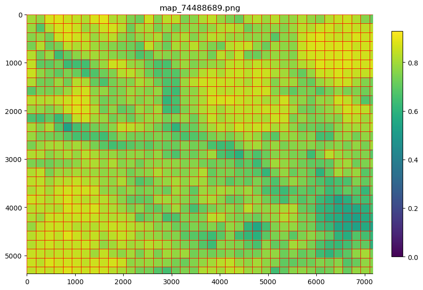
The show() and show_parent() methods can be used to plot these values ontop of your patches. This is done by specifying the column_to_plot argument.

e.g. to view “mean_pixel_R” on your patches:

#EXAMPLE
parent_list = my_files.list_parents()
my_files.show_parent(parent_list[0], column_to_plot="mean_pixel_R")

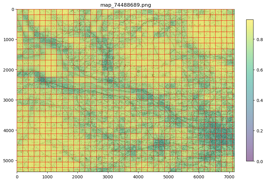
If you want to see your image underneath, you can specify the alpha argument, which sets the transparency of your plotted values. alpha can range between 0 and 1, with lower alpha values allowing you to see the more of the image underneath.

e.g. to view “mean_pixel_R” on your patches:

#EXAMPLE
parent_list = my_files.list_parents()
my_files.show_parent(parent_list[0], column_to_plot="mean_pixel_R", alpha=0.5)

Note

The column_to_plot argument can also be used with the show() method.

Advanced usage

Other arguments you may want to specify when showing your images (for both the show() and show_parent() methods):

plot_parent - By default, this is set to True so that the parent image is shown. If you would like to remove the parent image, e.g. if you are plotting column values, you can set plot_parent=False. This should speed up the code for plotting.
patch_border - By default, this is set to True so that borders are plotted around each patch. Setting patch_border to False (by specifying patch_border=False) will stop patch borders being shown.
border_color - By default, this is set to "r" (red). Any of the colors found here can be used instead.
cmap - By default, this is set to "viridis"`. Any of the color maps found here can be used instead.
plot_histogram - Setting this to True (by specifying plot_histogram=True) will result in a histogram of the values found in column_to_plot being produced.