Spot text
MapReader implements three frameworks for spotting text on maps:
DPTextDETRRunner- This is used to detect text on maps using DPTextDETR and outputs bounding boxes and scores.DeepSoloRunner- This is used to detect and recognize text on maps using DeepSolo and outputs bounding boxes, text and scores.MapTextPipeline- This is used to detect and recognize text on maps using MapTextPipeline and outputs bounding boxes, text and scores.
We recommend using the MapTextPipeline for most use cases as it has been used to train a model on a sample of David Rumsey maps and so should work best for map text spotting.
Installing dependencies
To run text spotting with MapReader, you will need to install the required dependencies. Refer to our installation instructions for guidance on how to install these.
Assuming your installation is successful, you will have installed the following:
Advice for patch size
When running the text spotting models, we recommend using a patch size of 1024x1024 pixels. This is the size used as input to the models, and so should give the best results.
You may also want to create some overlap between your patches as this should minimise cut off text at the edges of patches. MapReader has an algorithm to deduplicate overlapping bounding boxes so this creating an overlap will enable the fullest text to be detected. You will need to experiment with the amount of overlap to find the best results for your maps.
Note
Greater overlaps will create more patches and result in greater computational costs when running.
See the Load user guide for more information on how to create patches.
Set-up the runner
Once you have installed the dependencies, you can set up your chosen “runner”.
You will need to choose a model configuration and download the corresponding model weights.
Config files can be found in the
DPText-DETR,DeepSoloandMapTextPipelinerepositories under theconfigsdirectory.Weights files should be downloaded from the github repositories (links to the downloads are in the README).
e.g. for the DPTextDETRRunner, if you choose the “ArT/R_50_poly.yaml”, you should download the “art_final.pth” model weights file from the DPTextDETR repo.
e.g. for the DeepSoloRunner, if you choose the “R_50/IC15/finetune_150k_tt_mlt_13_15_textocr.yaml”, you should download the “ic15_res50_finetune_synth-tt-mlt-13-15-textocr.pth” model weights file from the DeepSolo repo.
e.g. for the MapTextRunner, if you choose the “ViTAEv2_S/rumsey/final_rumsey.yaml”, you should download the “rumsey-finetune.pth” model weights file from the MapTextPipeline repo.
Note
We recommend using the “ViTAEv2_S/rumsey/final_rumsey.yaml” configuration and “rumsey-finetune.pth” weights from the MapTextPipeline. But you should choose based on your own use case.
For the DPTextDETRRunner, use:
from mapreader import DPTextDETRRunner

#EXAMPLE
my_runner = DPTextDETR(
    "./patch_df.csv", # or .geojson
    "./parent_df.csv", # or .geojson
    cfg_file = "DPText-DETR/configs/DPText_DETR/ArT/R_50_poly.yaml",
    weights_file = "./art_final.pth",
)
or, if you have your patch_df and parent_df already loaded as pandas DataFrames or geopandas GeoDataFrames, you can use:
#EXAMPLE
my_runner = DPTextRunner(
    patch_df,
    parent_df,
    cfg_file = "DPText-DETR/configs/DPText_DETR/ArT/R_50_poly.yaml",
    weights_file = "./art_final.pth",
)
For the DeepSoloRunner, use:
from mapreader import DeepSoloRunner

#EXAMPLE
my_runner = DeepSoloRunner(
    patch_df,
    parent_df,
    cfg_file = "DeepSolo/configs/R_50/IC15/finetune_150k_tt_mlt_13_15_textocr.yaml",
    weights_file = "./ic15_res50_finetune_synth-tt-mlt-13-15-textocr.pth"
)
or, you can load your patch/parent dataframes from CSV/GeoJSON files as shown for the DPTextRunner (above).
For the MapTextRunner, use:
from mapreader import MapTextRunner

#EXAMPLE
my_runner = MapTextRunner(
    patch_df,
    parent_df,
    cfg_file = "MapTextPipeline/configs/ViTAEv2_S/rumsey/final_rumsey.yaml",
    weights_file = "./rumsey-finetune.pth"
)
or, you can load your patch/parent dataframes from CSV/GeoJSON files as shown for the DPTextRunner (above).
Note
You’ll need to adjust the paths to the config and weights files to match your own set-up!
By default, the runners will set the device to “cuda” if available, otherwise it will use “cpu”.
You can explicitly set this using the device argument:
#EXAMPLE
my_runner = MapTextRunner(
    "./patch_df.csv",
    "./parent_df.csv",
    cfg_file = "MapTextPipeline/configs/ViTAEv2_S/rumsey/final_rumsey.yaml",
    weights_file = "./rumsey-finetune.pth",
    device = "cuda",
)
Run the runner
You can then run the runner on all patches in your patch dataframe:
patch_preds = my_runner.run_all()
By default, this will return a dictionary containing all the predictions for each patch.
If you’d like to return a dataframe instead, use the return_dataframe argument:
patch_preds_df = my_runner.run_all(return_dataframe=True)
MapReader will automatically run a deduplication algorithm to remove overlapping bounding boxes, based on a minimum intersection of area (IoA) for each overlapping polygon. If two polygons overlap with intersection over area greater than the minimum IoA, the the one with the lower IoA will be kept (i.e. the larger of the two polygons).
Below are two examples of this:
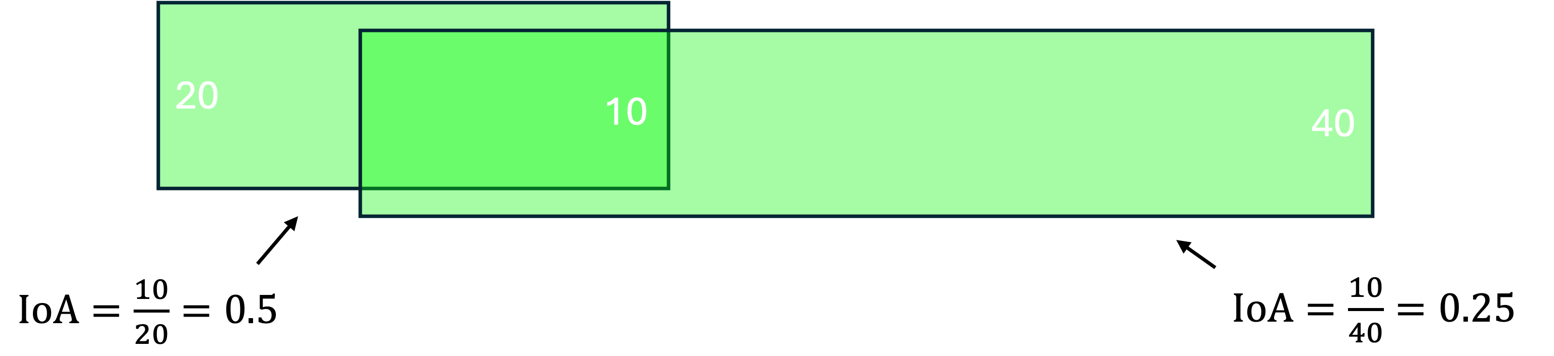
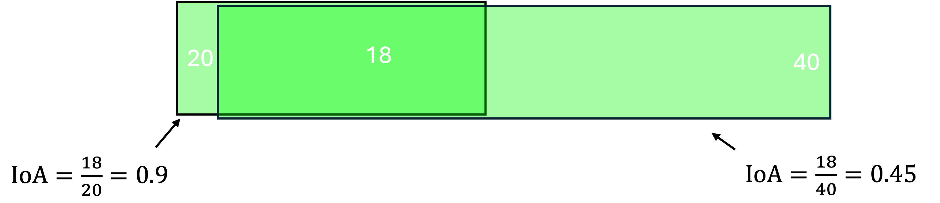
By default, the minimum IoA is set to 0.7 so the deduplication algorithm will only remove the smaller polygon in the second example.
You can adjust the minimum IoA by setting the min_ioa argument:
patch_preds_df = my_runner.run_all(return_dataframe=True, min_ioa=0.9)
Higher ``min_ioa``values will mean a tighter threshold for identifying two polygons as duplicates.
If you’d like to run the runner on a single patch, you can also just run on one image:
patch_preds = my_runner.run_on_image("path/to/your/image.png", min_ioa=0.7)
Again, this will return a dictionary by default but you can use the return_dataframe argument to return a dataframe instead.
To view the patch predictions, you can use the show_predictions method.
This takes an image ID as an argument, and will show you all the predictions for that image:
#EXAMPLE
my_runner.show_predictions(
    "patch-0-0-1000-1000-#map_74488689.png#.png"
)
By default, this will show the image with the bounding boxes drawn on in red and text in blue.
You can change these by setting the border_color and text_color arguments:
my_runner.show_predictions(
    "patch-0-0-1000-1000-#map_74488689.png#.png",
    border_color = "green",
    text_color = "yellow",
)
You can also change the size of the figure with the figsize argument.
Scale-up to whole map
Once you’ve got your patch-level predictions, you can scale these up to the parent image using the convert_to_parent_pixel_bounds method:
parent_preds = my_runner.convert_to_parent_pixel_bounds()
This will return a dictionary containing the predictions for the parent image.
If you’d like to return a dataframe instead, use the return_dataframe argument:
parent_preds_df = my_runner.convert_to_parent_pixel_bounds(return_dataframe=True)
If you have created patches with overlap, then you should deduplicate at the parent level as well.
You can do this by setting the deduplicate argument and passing a min_ioa value:
parent_preds_df = my_runner.convert_to_parent_pixel_bounds(return_dataframe=True, deduplicate=True, min_ioa=0.7)
This will help resolve any issues with predictions being cut-off at the edges of patches since the overlap should help find the full piece of text.
Again, to view the predictions, you can use the show_predictions method.
You should pass a parent image ID as the image_id argument:
#EXAMPLE
my_runner.show_predictions(
    "map_74488689.png"
)
As above, use the border_color, text_color and figsize arguments to customize the appearance of the image.
my_runner.show_predictions(
    "map_74488689.png",
    border_color = "green",
    text_color = "yellow",
    figsize = (20, 20),
)
Geo-reference
If you maps are georeferenced in your parent_df, you can also convert the pixel coordinates to georeferenced coordinates using the convert_to_coords method:
geo_preds_df = my_runner.convert_to_coords(return_dataframe=True)
Once this is done, you can use the explore_predictions method to view your predictions on a map.
For example, to view your predictions overlaid on an OpenStreetMap.Mapnik layer (the default), use:
my_runner.explore_predictions(
    "map_74488689.png",
)
Or, if your maps are taken from a tilelayer, you can specify the URL of the tilelayer you’d like to use as the base map:
my_runner.explore_predictions(
    "map_74488689.png",
    xyz_url="https://geo.nls.uk/mapdata3/os/6inchfirst/{z}/{x}/{y}.png"
)
You can also pass in a dictionary of style_kwargs to customize the appearance of the map.
Refer to the geopandas explore documentation for more information on the available options.
Saving
You can save your georeferenced predictions to a geojson file for loading into GIS software using the to_geojson method:
my_runner.to_geojson("text_preds.geojson")
This will save the predictions to a geojson file, with each text prediction as a separate feature.
By default, the geometry column will contain the polygon representing the bounding box of your text.
If instead you would like to save just the centroid of this polygon, you can set the centroid argument:
my_runner.to_geojson("text_preds.geojson", centroid=True)
This will save the centroid of the bounding box as the geometry column and create a “polygon” column containing the original polygon.
At any point, you can also save your patch, parent and georeferenced predictions to CSV files using the to_csv method:
my_runner.to_csv("my_preds/")
This will create a folder called “my_preds” and save the patch, parent and georeferenced predictions to CSV files within it.
As above, you can use the centroid=True argument to save the centroid of the bounding box instead of the full polygon.
Loading
If you have saved your predictions and want to reload them into a runner, you use either of the load_geo_predictions or load_patch_predictions methods.
Note
These methods will overwrite any existing predictions in the runner. So if you want to keep your existing predictions, you should save them to a file first!
The load_geo_predictions method is used to load georeferenced predictions from a geojson file:
my_runner.load_geo_predictions("text_preds.geojson")
Loading this will populate the patch, parent and georeferenced predictions in the runner.
The load_patch_predictions method is used to load patch predictions from a CSV file or pandas DataFrame.
To load a CSV file, you can use:
my_runner.load_patch_predictions("my_preds/patch_preds.csv")
Or, to load a pandas DataFrame, you can use:
my_runner.load_patch_predictions(patch_preds_df)
This will populate the patch and parent predictions in the runner but not the georeferenced predictions (in case you do not have georefencing information).
If you do want to convert your text predictions from pixel coordinates to geospatial coordinates, you can use the convert_to_coords method as shown above.
Search predictions
If you are using the DeepSoloRunner or the MapTextRunner, you will have recognized text outputs.
You can search these predictions using the search_preds method:
search_results = my_runner.search_preds("search term")
e.g To find all predictions containing the word “church” and ignoring the case:
# EXAMPLE
search_results = my_runner.search_preds("church")
By default, this will return a dictionary containing the search results.
If you’d like to return a dataframe instead, use the return_dataframe argument:
# EXAMPLE
search_results_df = my_runner.search_preds("church", return_dataframe=True)
You can also ignore the case of the search term by setting the ignore_case argument:
# EXAMPLE
search_results_df = my_runner.search_preds("church", return_dataframe=True, ignore_case=True)
The search accepts regex patterns so you can use these to search for more complex patterns.
e.g. To search for all predictions containing the word “church” or “chapel”, you could use the pattern “church|chapel”:
# EXAMPLE
search_results_df = my_runner.search_preds("church|chapel", return_dataframe=True, ignore_case=True)
Once you have your search results, you can view them on your map using the show_search_results method.
my_runner.show_search_results("map_74488689.png")
This will show the map with the search results.
As with the show_predictions method, you can use the border_color, text_color and figsize arguments to customize the appearance of the image.
If your maps are georeferenced, you can also use the explore_search_results method to view your search results on a map.
This method works in the same way as the explore_predictions method.
So, for example, to show your search results overlaid on your chosen tilelayer, you can use:
my_runner.explore_search_results(
    "map_74488689.png",
    xyz_url="https://geo.nls.uk/mapdata3/os/6inchfirst/{z}/{x}/{y}.png"
)
You can also pass in a dictionary of style_kwargs to customize the appearance of the map.
Save search results
If your maps are georeferenced, you can also save your search results using the search_results_to_geojson method:
my_runner.search_results_to_geojson("search_results.geojson")
This will save the search results to a geojson file, with each search result as a separate feature which can be loaded into GIS software for further analysis/exploration.
If, however, your maps are not georeferenced, you will need to save the search results to a csv file using the pandas to_csv method:
search_results_df.to_csv("search_results.csv")